Designing Data-Intensive Applications

Part 1: Foundation of Data systems

• Chapter 1: Reliable, Scalable, and Maintainable Applications
• Chapter 2: Data Models and Query Languages
• Chapter 3: Storage and Retrieval
• Chapter 4: Encoding and Evolution

• Chapter 5: Replication
• Chapter 6: Partitioning
• Chapter 7: Transactions
• Chapter 8: The Trouble with Distributed Systems
• Chapter 9: Consistency and Consensus

• Chapter 10: Batch Processing
• Chapter 11: Stream Processing
• Chapter 12: The Future of Data Systems

Chapter 2: Data Models and Query Languages

Reasons to adopt NoSQL over relational data stores:

• A need for greater scalability than relational databases can easily achieve, including very large datasets or very high write throughput
• A widespread preference for free and open source software over commercial database products
• Specialized query operations that are not well supported by the relational model
• Frustration with the restrictiveness of relational schemas, and a desire for a more dynamic and expressive data model

With document stores, the work of making joins is shifted from the db to the app code

Impedance mismatch is the disconnect between object in app code and the db model of tables. ORMs help but they can’t completely hide the differences between the two models.

Historically, data started out being represented as one big tree (the hierarchical model), but that wasn’t good for representing many-to-many relationships, so the relational model was invented to solve that problem. More recently, developers found that some applications don’t fit well in the relational model either. New nonrelational “NoSQL” datastores have diverged in two main directions:

1. Document databases target use cases where data comes in self-contained documents and relationships between one document and another are rare.
2. Graph databases go in the opposite direction, targeting use cases where anything is potentially related to everything.

All three models (document, relational, and graph) are widely used today, and each is good in its respective domain. One model can be emulated in terms of another model—for example, graph data can be represented in a relational database—but the result is often awkward. That’s why we have different systems for different purposes, not a single one-size-fits-all solution.

One thing that document and graph databases have in common is that they typically don’t enforce a schema for the data they store, which can make it easier to adapt applications to changing requirements. However, your application most likely still assumes that data has a certain structure; it’s just a question of whether the schema is explicit (enforced on write) or implicit (assumed on read).

Chapter 3: Storage and Retrieval

Why should you, as an application developer, care how the database handles storage and retrieval internally? You’re probably not going to implement your own storage engine from scratch, but you do need to select a storage engine that is appropriate for your application, from the many that are available. In order to tune a storage engine to perform well on your kind of workload, you need to have a rough idea of what the storage engine is doing under the hood.

In particular, there is a big difference between storage engines that are optimized for transactional workloads and those that are optimized for analytics.

OLTP - Online Transaction Processing OLAP - Online Analytics Processing

OLTP vs OLAP

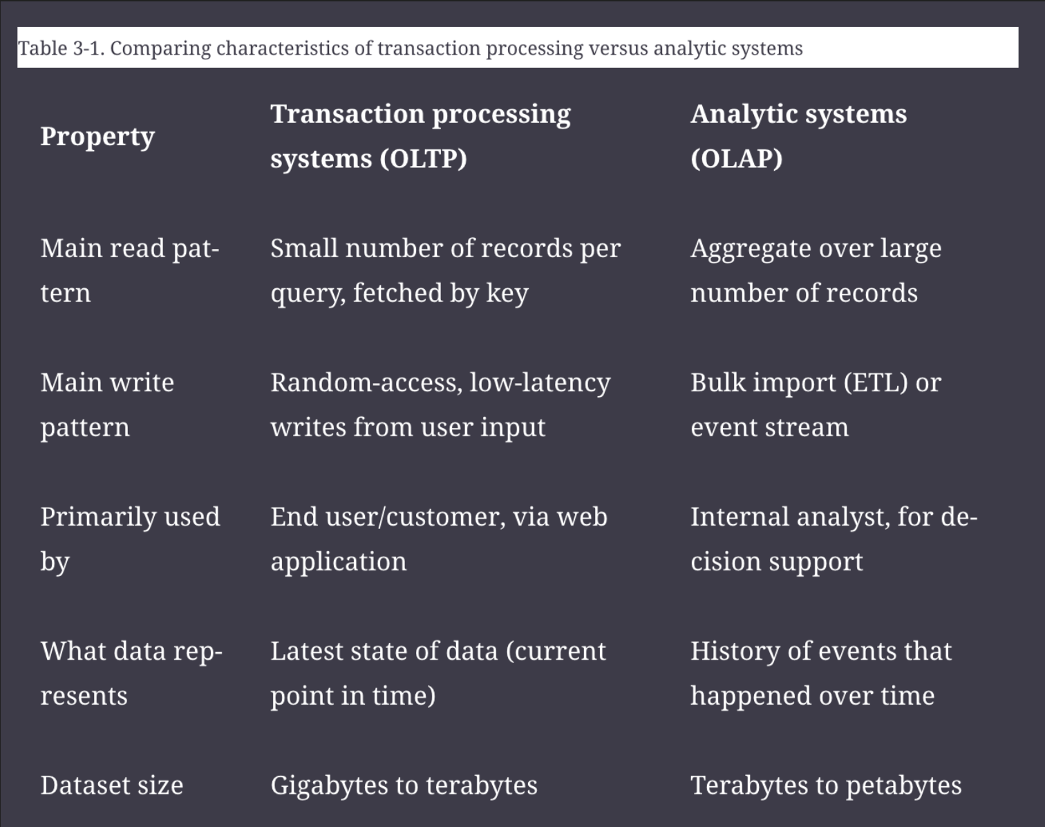
Disk seek time is often the biggest bottleneck when using OLTP databases. Disk bandwidth is often the biggest bottleneck when using OLAP databases.

OLTP

Storage engines

Log structured

This storage strategy only permits appending to files and deleting obsolete files. A file that has been written is never updated.

Sequential writes on disk enables higher write throughput compared to random-access writes.

Examples:

• SSTables
• LSM-trees
• LevelDB
• Cassandra
• HBase
• Lucene
• Bitcask

Update-in-place

Treat the disk as a set of fix-sized pages that can be overwritten.

B-trees are the most common example of this philosophy.

Database indexes

An index is an additional structure that is derived from the primary data. Many databases allow you to add and remove indexes, and this doesn’t affect the contents of the database; it only affects the performance of queries.

A big downside to using indexes is the overhead incurred on write operations. It's hard to beat the performance of simply appending to a file because that’s the simplest possible write operation. The index needs to be updated every time data is written which slows down writes.

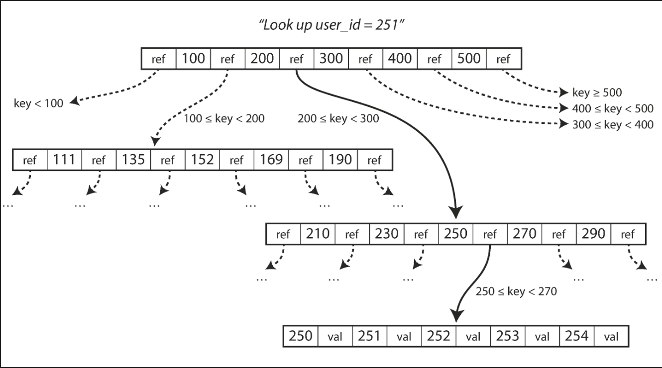
B-trees are the most widely used indexing structure.

Introduced in 1970 and called “ubiquitous” less than 10 years later, B-trees have stood the test of time very well. They remain the standard index implementation in almost all relational databases, and many nonrelational databases use them too.

B-tree diagram:

In-memory databases

Counterintuitively, the performance advantage of in-memory databases is not due to the fact that they don’t need to read from disk. Even a disk-based storage engine may never need to read from disk if you have enough memory, because the operating system caches recently used disk blocks in memory anyway. Rather, they can be faster because they can avoid the overheads of encoding in-memory data structures in a form that can be written to disk.

OLAP

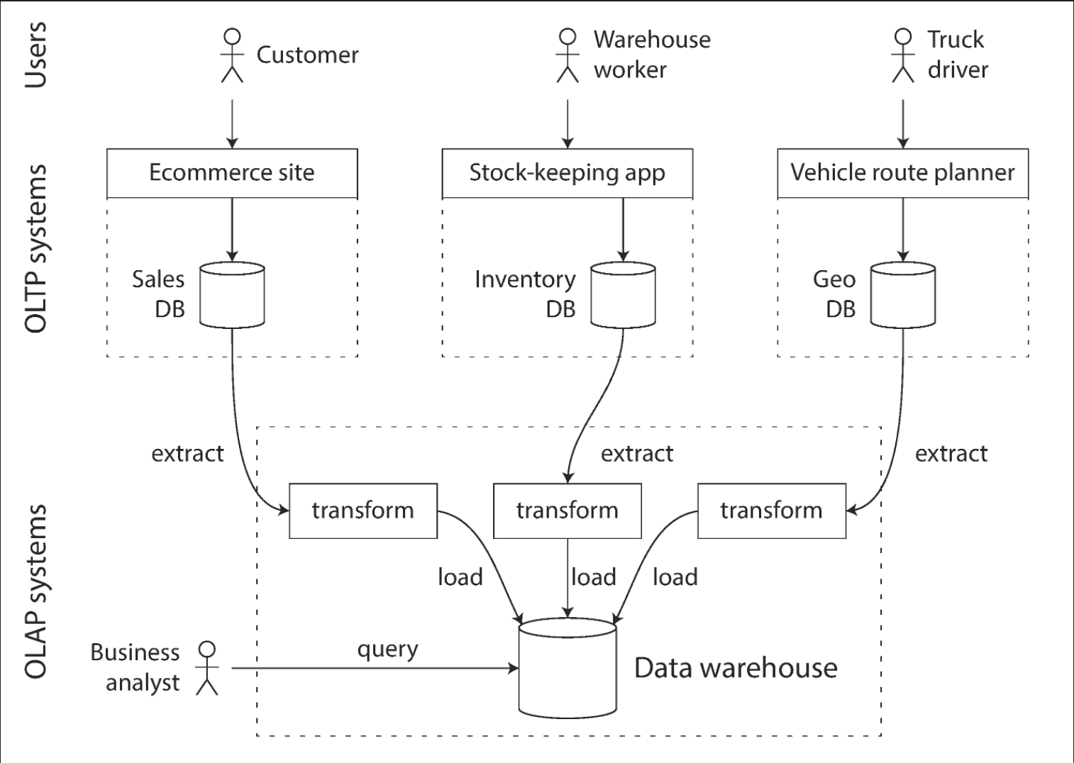
OLTP databases usually aren't used for business analysts to run ad hoc analytics queries.

These queries are often expensive (scanning large parts of the dataset) which can harm the performance of concurrently executing transactions. Separate "data warehouse" databases are for running these analytics queries.

ETL jobs will get data dumps or data streams from OLTP databases, massage the data into an analysis-friendly schema and store the data in the warehouse.

Data models for data warehousing

Star schema aka dimensional modeling

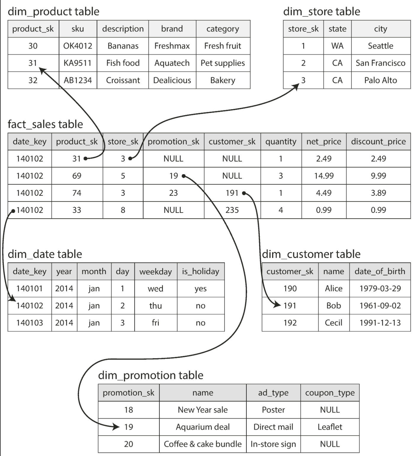
Each row of a fact table represents an event. Dimensions represent the who, what , when, where, why and how of the event.

Snowflake schema Similar to a star schema but dimensions are broken down into sub-dimensions. Snowflake schemas are more normalized than star schemas, but star schemas are often preferred because they are simpler for analysts to work with.

Regardless of schema design, most OLAP databases leverage column-oriented storage. The idea is to store all the values from each column together instead of storing all the values from each row. This makes queries more efficient for tables with hundreds of columns that may not be necessary to process in order to fulfill the query.

There are also column-oriented compression and sorting techniques used to improve read performance. LSM-trees are commonly used for write operations.

Chapter 4: Encoding and Evolution

With a bit of care, backward/forward compatibility and rolling upgrades are very much achievable.

Encoding

Whenever you want to send some data to another process with which you don’t share memory (e.g. whenever you want to send data over the network or write it to a file) you need to encode it as a sequence of bytes. This chapter covers a variety of encodings for doing this.

The translation from the in-memory representation to a byte sequence is called encoding (also known as serialization or marshalling), and the reverse is called decoding (parsing, deserialization, unmarshalling).

Note: Serialization is perhaps a more common term than encoding but it is also used in the context of transactions with a completely different meaning.

Types of encoding:

• Language-specific formats
• JSON and XML
• Binary encoding
• Thrift and Protocol Buffers
• Avro

Language-specific formats

Generally a bad idea to use due to language specificity, security issues, data versioning/backward compatibility complexity and efficiency problems.

JSON, XML and binary variants

There is a lot of ambiguity around the encoding of numbers.

In XML and CSV, unless you refer to an external schema you cannot distinguish between a number and a string that happens to consist of digits.

JSON distinguishes strings and numbers but it doesn’t distinguish integers and floating-point numbers. Also it doesn’t specify any precision.

This is a problem when dealing with large numbers. For example, integers greater than 253 cannot be exactly represented in an IEEE 754 double-precision floating-point number, so such numbers become inaccurate when parsed in a language that uses floating-point numbers (e.g. JavaScript).

An example of numbers larger than 253 occurs on Twitter, which uses a 64-bit number to identify each tweet. The JSON returned by Twitter’s API includes tweet IDs twice, once as a JSON number and once as a decimal string, to work around the fact that the numbers are not correctly parsed by JavaScript applications

There's optional schema support for both XML and JSON. These schema languages are quite powerful but quite complicated to learn and implement. Use of XML schemas is much more widespread than JSON schemas. Since the correct interpretation of data (e.g. numbers and binary strings) depends on information in the schema, applications that don’t use XML/JSON schemas need to potentially hardcode the appropriate encoding/decoding logic instead.

JSON and XML have good support for Unicode character strings (i.e., human-readable text), but they don’t support binary strings (sequences of bytes without a character encoding). Folks get around this limitation by encoding the binary data as text using Base64. A schema is then used to indicate that the value should be interpreted as Base64-encoded. This works, but it’s somewhat of a hack and it increases the data size by 33%.

Despite these flaws, JSON and XML are good enough for many purposes. It’s likely that they will remain popular, especially as data interchange formats (i.e. for sending data from one organization to another). In these situations, as long as people agree on what the format is, it often doesn’t matter how pretty or efficient the format is.

Thrift and Protocol Buffers

These binary schema–driven formats allow compact, efficient encoding with clearly defined forward and backward compatibility semantics. The schemas can be useful for documentation and code generation in statically typed languages. However, these formats have the downside that data needs to be decoded before it is human-readable.

What about backward compatibility? As long as each field has a unique tag number, new code can always read old data, because the tag numbers still have the same meaning. The only detail is that if you add a new field, you cannot make it required. If you were to add a field and make it required, that check would fail if new code read data written by old code, because the old code will not have written the new field that you added. Therefore, to maintain backward compatibility, every field you add after the initial deployment of the schema must be optional or have a default value.

A curious detail of Protocol Buffers is that it does not have a list or array datatype. Instead, it has a repeated marker for fields (which is a third option alongside required and optional). A repeated field indicates that the same field tag simply appears multiple times in the record. This has the nice effect that it’s okay to change an optional (single-valued) field into a repeated (multi-valued) field. New code reading old data sees a list with zero or one elements (depending on whether the field was present). Old code reading new data sees only the last element of the list.

Data flow

Some of the most common ways how data flows between processes:

• databases
• service calls
• asynchronous message passing

Databases

The process writing to the database encodes the data and the process reading from the database decodes it.

Service calls

RPC and REST APIs, where the client encodes a request, the server decodes the request and encodes a response, and the client finally decodes the response.

The API of a SOAP web service is described using an XML-based language called the Web Services Description Language, or WSDL. WSDL enables code generation so that a client can access a remote service using local classes and method calls (which are encoded to XML messages and decoded again by the framework). This is useful in statically typed programming languages, but less so in dynamically typed ones (see “Code generation and dynamically typed languages”).

As WSDL is not designed to be human-readable, and as SOAP messages are often too complex to construct manually, users of SOAP rely heavily on tool support, code generation, and IDEs [38]. For users of programming languages that are not supported by SOAP vendors, integration with SOAP services is difficult.

Custom RPC protocols with a binary encoding format can achieve better performance than something generic like JSON over a REST service call. However, a RESTful API has other significant advantages:

• it is good for experimentation and debugging - you can simply make requests to it using a web browser or the command-line tool curl, without any code generation or software installation
• it is supported by all mainstream programming languages and platforms, and there is a vast ecosystem of tools available - servers, caches, load balancers, proxies, firewalls, monitoring, debugging tools, testing tools, etc.

RPC frameworks are often used for calls between services owned by the same organization, typically within the same datacenter.

Message passing

Nodes communicate by sending each other messages that are encoded by the sender and decoded by the recipient.

Using a message broker has several advantages over direct RPC:

• It can act as a buffer if the recipient is unavailable or overloaded which improves system reliability.
• It can automatically redeliver messages to a process that has crashed which prevents messages from being lost.
• It avoids the sender needing to know the IP address and port number of the recipient. - Particularly useful in a cloud deployment where virtual machines often come and go.
• It allows one message to be sent to several recipients.
• It logically decouples the sender from the recipient. - The sender just publishes messages and doesn’t care who consumes them.

However, message-passing communication is usually one-way. A sender normally doesn’t expect to receive a reply to its messages. It is possible for a process to send a response but it would usually be done via a separate channel.

Part 2: Distributed Data

There are several reasons why you might want to replicate data:

• keep data geographically close to your users
  • reduces access latency
• allow the system to continue working even if some of its parts have failed
  • increases availability / fault tolerance
• scale out the number of machines that can serve read queries
  • increases read throughput / scalability

If your data is distributed across multiple nodes, you need to be aware of the constraints and trade-offs that occur in such a distributed system—the database cannot magically hide these from you.

2 common ways data is distributed across multiple nodes:

• Replication - Keeping a copy of the same data on several different nodes, potentially in different locations. - Replication provides redundancy: if some nodes are unavailable, the data can still be served from the remaining nodes. - Replication can also help improve performance.
• Partitioning - Splitting a big database into smaller subsets called partitions so that different partitions can be assigned to different nodes (also known as sharding).

Node failures, unreliable networks, and trade-offs around replica consistency, durability, availability, and latency are fundamental problems in distributed systems.

Chapter 5: Replication

All of the difficulty in replication lies in handling changes to replicated data. Three popular algorithms for replicating changes between nodes are single-leader, multi-leader, and leaderless replication.

Single-leader replication

Clients send all writes to a single node (the leader), which sends a stream of data change events to the other replicas (followers). Reads can be performed on any replica, but reads from followers might be stale.

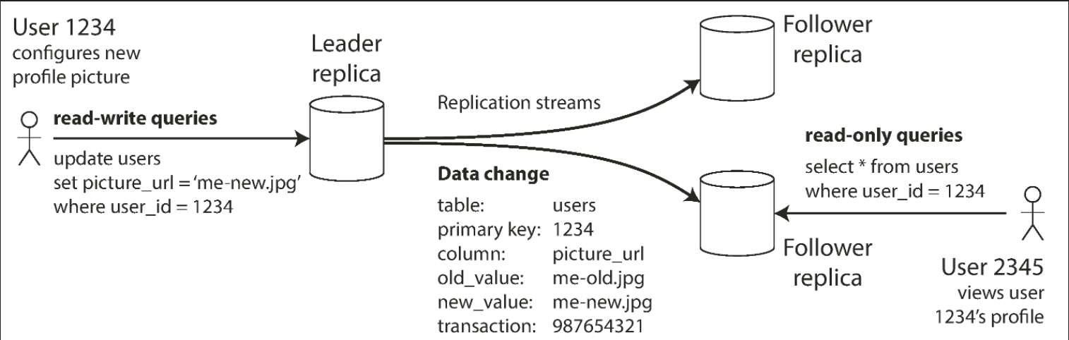
This approach is popular because it's relatively easy to understand and there is no conflict resolution to worry about.

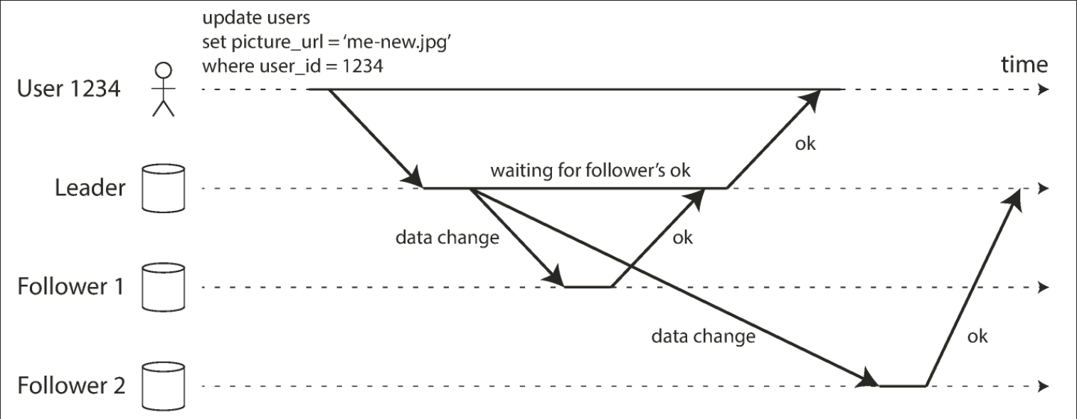
The advantage of synchronous replication is that the follower is guaranteed to have an up-to-date copy of the data that is consistent with the leader. If the leader suddenly fails, we can be sure that the data is still available on the follower. The disadvantage is that if the synchronous follower doesn’t respond (because it has crashed, or there is a network fault, or for any other reason), the write cannot be processed. The leader must block all writes and wait until the synchronous replica is available again.

If you enable synchronous replication on a database it usually means that one of the followers is synchronous and the others are asynchronous. If the synchronous follower becomes unavailable or slow, one of the asynchronous followers is made synchronous. This guarantees that you have an up-to-date copy of the data on at least two nodes (the leader and one synchronous follower). This configuration is sometimes also called semi-synchronous.

The figure below represents leader-based replication with one synchronous and one asynchronous follower.

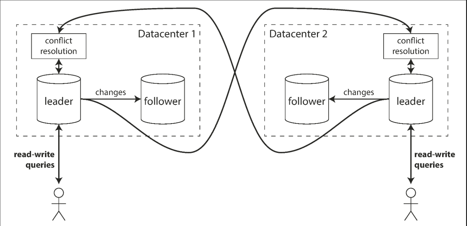
Multi-leader replication

Clients send each write to one of several leader nodes, any of which can accept writes. The leaders send streams of data change events to each other and to any follower nodes.

This approach can be more robust in the presence of faulty nodes, network interruptions and latency spikes. This comes at the cost of being harder to reason about as well as the cost of very weak consistency guarantees.

The figure below outlines an approach for multi-leader replication across multiple data centers.

Leaderless replication

Clients send each write to several nodes, and read from several nodes in parallel in order to detect and correct nodes with stale data.

Eventual consistency models

There are a few consistency models which are helpful for deciding how an application should behave under replication lag:

Read-after-write consistency

Users should always see data that they submitted themselves. This consistency model makes no promises about other users' updates being visible in real time.

Cross-device read-after-write consistency ensures that if the user enters some information on one device and then views it on another device, they should see the information they just entered.

Monotonic reads

After users have seen the data at one point in time, they shouldn’t later see the data from some earlier point in time.

In the figure below, a user first reads from a fresh replica, then from a stale replica. Time appears to go backward. To prevent this anomaly, we need monotonic reads.

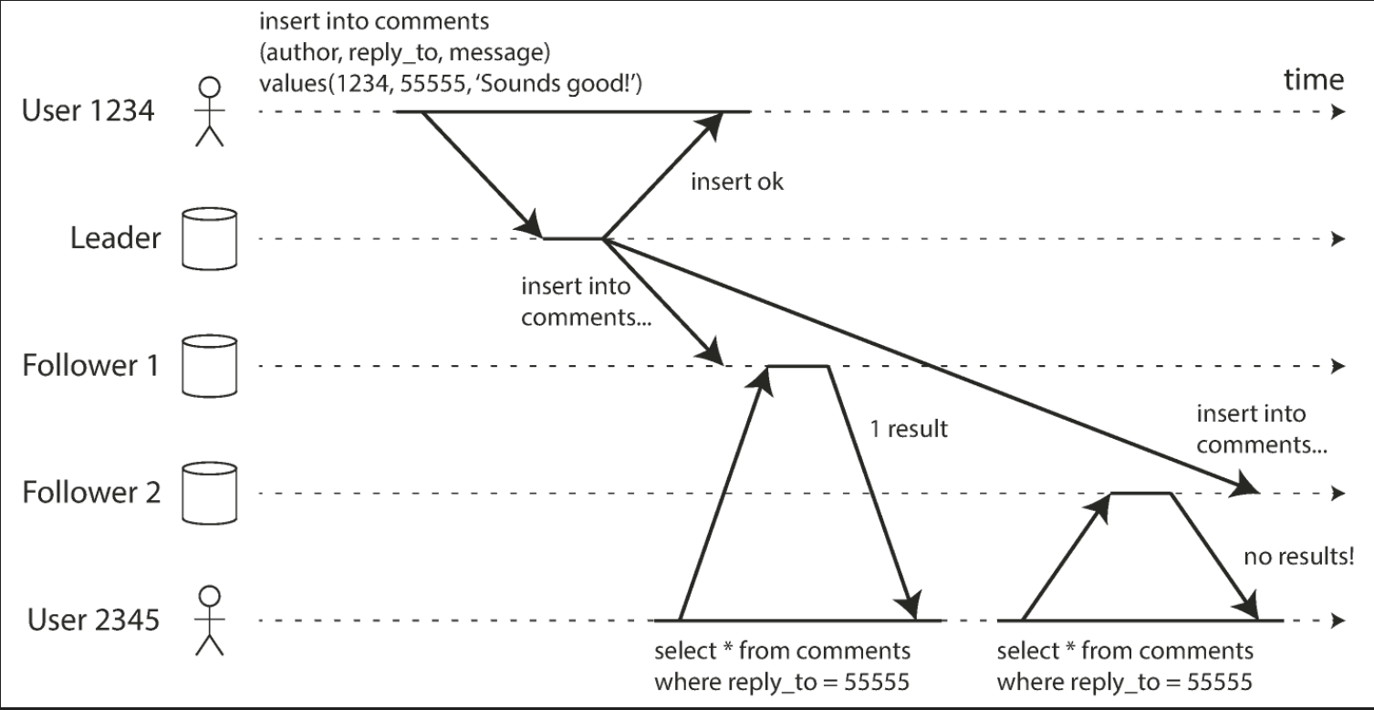
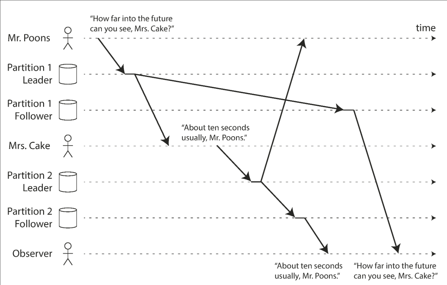
Consistent prefix reads

Users should see the data in a state that makes causal sense: for example, seeing a question and its reply in the correct order.

If some partitions are replicated slower than others, an observer may see the answer before they see the question. The figure below demonstrates this scenario.

Chapter 6: Partitioning

Partitioning is necessary when you have so much data that storing and processing it on a single machine is no longer feasible.

The goal of partitioning is to spread the data and query load evenly across multiple machines, avoiding hot spots (nodes with disproportionately high load). This requires choosing a partitioning scheme that is appropriate to your data, and rebalancing the partitions when nodes are added to or removed from the cluster.

Main approaches to partitioning:

• Key range partitioning
• Hash partitioning

Key range partitioning

Keys are sorted and a partition owns all the keys from some minimum up to some maximum. Sorting has the advantage that efficient range queries are possible but there is a risk of hot spots if the application often accesses keys that are close together in the sorted order.

In this approach, partitions are typically rebalanced dynamically by splitting the range into two subranges when a partition gets too big.

Hash partitioning

A hash function is applied to each key and a partition owns a range of hashes. This method destroys the ordering of keys which makes range queries inefficient but may distribute load more evenly.

When partitioning by hash it's common to create a fixed number of partitions in advance, to assign several partitions to each node, and to move entire partitions from one node to another when nodes are added or removed. Dynamic partitioning can also be used.

Partitioning and secondary indexes

A secondary index also needs to be partitioned, and there are two methods:

1. Document-partitioned indexes
2. Term-partitioned indexes

Document-partitioned indexes (local indexes)

The secondary indexes are stored in the same partition as the primary key and value. This means that only a single partition needs to be updated on write, but a read of the secondary index requires a scatter/gather across all partitions.

Term-partitioned indexes (global indexes)

The secondary indexes are partitioned separately, using the indexed values. An entry in the secondary index may include records from all partitions of the primary key. When a document is written, several partitions of the secondary index need to be updated; however, a read can be served from a single partition.

Routing

Techniques for routing queries to the appropriate partition range from simple partition-aware load balancing to sophisticated parallel query execution engines.

By design, every partition operates mostly independently which allows a partitioned database to scale to multiple machines.

However, operations that need to write to several partitions can be difficult to reason about. For example, what happens if the write to one partition succeeds, but another fails?

Chapter 7: Transactions

A transaction is a way for an application to group several reads and writes together into a logical unit.

An application with very simple access patterns can probably manage without transactions. For example, reading and writing only a single record.

For more complex apps, the following error scenarios could cause data to become inconsistent.

• processes crashing
• network interruptions
• power outages
• disk full
• unexpected concurrency

Transactions eliminate the need to think about these potential error cases.

Concurrency control

Widely used isolation levels:

• read committed
• snapshot isolation (sometimes called repeatable read)
• serializable

These isolation levels can be characterized by discussing various examples of race conditions:

• dirty reads
• dirty writes
• read skew
• lost updates
• write skew
• phantom reads

Dirty reads

One client reads another client’s writes before they have been committed. The read committed isolation level and stronger levels prevent dirty reads.

Dirty writes

One client overwrites data that another client has written, but not yet committed. Almost all transaction implementations prevent dirty writes.

Read skew

A client sees different parts of the database at different points in time. Some cases of read skew are also known as nonrepeatable reads. This issue is most commonly prevented with snapshot isolation, which allows a transaction to read from a consistent snapshot corresponding to one particular point in time. It is usually implemented with multi-version concurrency control (MVCC).

Lost updates

Two clients concurrently perform a read-modify-write cycle. One overwrites the other’s write without incorporating its changes, so data is lost. Some implementations of snapshot isolation prevent this anomaly automatically, while others require a manual lock (SELECT FOR UPDATE).

Write skew

A transaction reads something, makes a decision based on the value it saw, and writes the decision to the database. However, by the time the write is made, the premise of the decision is no longer true. Only serializable isolation prevents this anomaly.

Phantom reads

A transaction reads objects that match some search condition. Another client makes a write that affects the results of that search. Snapshot isolation prevents straightforward phantom reads, but phantoms in the context of write skew require special treatment, such as index-range locks.

Serializable transactions

Weak isolation levels protect against some of those anomalies but leave you, the application developer, to handle others manually (e.g., using explicit locking). Only serializable isolation protects against all of these issues.

Approaches to implementing serializable transactions:

• Literally executing transactions in a serial order
• Two-phase locking
• Serializable snapshot isolation (SSI)

Literally executing transactions in a serial order

If you can make each transaction very fast to execute, and the transaction throughput is low enough to process on a single CPU core, this is a simple and effective option.

Two-phase locking

For decades this has been the standard way of implementing serializability, but many applications avoid using it because of its performance characteristics.

Serializable snapshot isolation (SSI)

A fairly new algorithm that avoids most of the downsides of the previous approaches. It uses an optimistic approach, allowing transactions to proceed without blocking. When a transaction wants to commit, it is checked, and it is aborted if the execution was not serializable.

Chapter 8: The Trouble with Distributed Systems

If you can simply keep things on a single machine, it is generally worth doing so.

Scalability is not the only reason for wanting to use a distributed system. Fault tolerance and low latency (by placing data geographically close to users) are equally important goals, and those things cannot be achieved with a single node.

Partial failures

The defining characteristic of distributed systems is the fact that they can have partial failures.

Some problems that can occur in distributed systems:

• Sending packets over the network may be lost or arbitrarily delayed. - Likewise, the reply may be lost or delayed. - If you don’t get a reply you have no idea whether the message got through.
• A node’s clock may be significantly out of sync with other nodes. - It may suddenly jump forward or back in time. - Relying on it is dangerous.
• A process may pause for a substantial amount of time at any point in its execution. - For example, due to a stop-the-world garbage collector. - Paused processes may also be declared dead by other nodes and then come back to life again without realizing that it was paused.

Whenever software tries to do anything involving other nodes there is the possibility that it may:

• occasionally fail
• randomly slow down
• not respond at all (and eventually time out)

Fault tolerance

In distributed systems fault tolerance allows the system as a whole to continue functioning even when some of its constituent parts are broken.

The first step is to detect the faults which isn't easy.

Most systems rely on timeouts to determine whether a remote node is still available. Timeouts can’t distinguish between network and node failures. Variable network delay sometimes causes a node to be falsely suspected of crashing.

Once a fault is detected, making a system tolerate it is not easy either since there is no shared state between the machines. Major decisions cannot be safely made by a single node. Instead we require protocols that enlist help from other nodes and try to get a quorum to agree via message passing over a network.

Unreliability of networks, clocks, and processes is avoidable. It's possible to give hard real-time response guarantees and bounded delays in networks. However, doing so is very expensive and results in lower utilization of hardware resources. Most non-safety-critical systems choose cheap and unreliable over expensive and reliable.

Chapter 9: Consistency and Consensus

Consistency models

Linearizability

Linearizability is a popular consistency model. Its goal is to make replicated data appear as though there were only a single copy, and to make all operations act on it atomically.

Linearizability makes a database behave like a variable in a single-threaded program. It's appealing because it's easy to understand but it has the downside of being slow, especially in environments with large network delays.

Causality

Causality imposes an ordering on events in a system (what happened before what, based on cause and effect).

Unlike linearizability which puts all operations in a single, ordered timeline, causality provides us with a weaker consistency model. Some things can be concurrent so the version history is like a timeline with branching and merging.

Causal consistency does not have the coordination overhead of linearizability and is much less sensitive to network problems.

Causality is not a silver bullet. There are limitations. Not all things can be implemented this way.

Consider an example of ensuring that a username is unique and rejecting concurrent registrations for the same username. If one node is going to accept a registration, it needs to somehow know that another node isn’t concurrently in the process of registering the same name.

We can solve this problem with consensus.

Consensus

Achieving consensus means deciding something in such a way that all nodes agree on what was decided and the decision is irrevocable.

Not every system necessarily requires consensus. For example, leaderless and multi-leader replication systems typically do not use global consensus.

Tools like ZooKeeper play an important role in providing an “outsourced” consensus, failure detection, and membership service that applications can use. It’s not easy to use, but it is much better than trying to develop your own algorithms that can withstand all the potential problems. If you find yourself wanting to do one of those things that is reducible to consensus, and you want it to be fault-tolerant, then it is advisable to use something like ZooKeeper.

A wide range of problems are actually reducible to consensus and are equivalent to each other (if you have a solution for one of them, you can easily transform it into a solution for one of the others). Such problems include:

Linearizable compare-and-set registers

The register needs to atomically decide whether to set its value, based on whether its current value equals the parameter given in the operation.

Atomic transaction commit

A database must decide whether to commit or abort a distributed transaction.

Total order broadcast

The messaging system must decide on the order in which to deliver messages.

Locks and leases

When several clients are racing to grab a lock or lease, the lock decides which one successfully acquired it.

Membership/coordination service

Given a failure detector (e.g., timeouts), the system must decide which nodes are alive, and which should be considered dead because their sessions timed out.

Uniqueness constraint

When several transactions concurrently try to create conflicting records with the same key, the constraint must decide which one to allow and which should fail with a constraint violation.

Single-leader databases

All of these are straightforward if you only have a single node or if you are willing to assign the decision-making capability to a single node.

This is what happens in a single-leader database. All the power to make decisions is vested in the leader. This is why single-leader databases are able to provide linearizable operations, uniqueness constraints, a totally ordered replication log, and more.

However, if that single leader fails, or if a network interruption makes the leader unreachable such a system becomes unable to make any progress. There are three ways of handling that situation:

1. Wait for the leader to recover and accept that the system will be blocked in the meantime.
   • This approach does not fully solve consensus because it does not satisfy the termination property (if the leader does not recover, the system can be blocked forever).
2. Manually fail over by getting humans to choose a new leader node and reconfigure the system to use it.
   • Many relational databases take this approach.
   • The speed of failover is limited by the speed at which humans can act which is generally slower than computers.
3. Use an algorithm to automatically choose a new leader.
   • This approach requires a consensus algorithm and it should handle adverse network conditions.

Although a single-leader database can provide linearizability without executing a consensus algorithm on every write, it still requires consensus to maintain its leadership and for leadership changes. In some sense, having a leader only “kicks the can down the road”. Consensus is still required, only in a different place and less frequently.

Part 3: Derived Data

Up until this part of the book there was an assumption that there was only one database in the application.

In practice, applications commonly use a combination of several different data stores, caches, analytics systems, etc. These applications implement mechanisms for moving data from one store to another.

Systems that store and process data can be grouped into two generic categories:

• Systems of record

  A system of record, also known as source of truth, holds the authoritative version of your data. When new data comes in, e.g., as user input, it is first written here. Each fact is represented exactly once (the representation is typically normalized). If there is any discrepancy between another system and the system of record, then the value in the system of record is (by definition) the correct one.

• Derived data systems

  Data in a derived system is the result of taking some existing data from another system and transforming or processing it in some way. If you lose derived data, you can recreate it from the original source. A classic example is a cache: data can be served from the cache if present, but if the cache doesn’t contain what you need, you can fall back to the underlying database. Denormalized values, indexes, and materialized views also fall into this category. In recommendation systems, predictive summary data is often derived from usage logs.

Part 3 examines the issues around integrating multiple different data systems into one coherent application architecture. These data systems potentially have different data models and are optimized for different access patterns.

The data integration problem that arises can be solved by using batch processing and event streams to let data changes flow between different systems.

Certain systems are designated as systems of record and other data is derived from them through transformations. We can maintain indexes, materialized views, machine learning models, statistical summaries, etc.

A problem in one area is prevented from spreading to unrelated parts of the system by making these derivations and transformations asynchronous and loosely coupled. This increases the robustness and fault-tolerance of the system as a whole.

Chapter 10: Batch Processing

A system cannot be successful if it is too strongly influenced by a single person. Once the initial design is complete and fairly robust, the real test begins as people with many different viewpoints undertake their own experiments.

Donald Knuth

Three different types of systems:

• Services (online systems)

  A service waits for a request or instruction from a client to arrive. When one is received, the service tries to handle it as quickly as possible and sends a response back. Response time is usually the primary measure of performance of a service, and availability is often very important (if the client can’t reach the service, the user will probably get an error message).

• Batch processing systems (offline systems)

  A batch processing system takes a large amount of input data, runs a job to process it, and produces some output data. Jobs often take a while (from a few minutes to several days), so there normally isn’t a user waiting for the job to finish. Instead, batch jobs are often scheduled to run periodically (for example, once a day). The primary performance measure of a batch job is usually throughput (the time it takes to crunch through an input dataset of a certain size). We discuss batch processing in this chapter.

• Stream processing systems (near-real-time systems)

  Stream processing is somewhere between online and offline/batch processing (so it is sometimes called near-real-time or nearline processing). Like a batch processing system, a stream processor consumes inputs and produces outputs (rather than responding to requests). However, a stream job operates on events shortly after they happen, whereas a batch job operates on a fixed set of input data. This difference allows stream processing systems to have lower latency than the equivalent batch systems. As stream processing builds upon batch processing, we discuss it in Chapter 11.

Even if various tasks have to be retried, a batch processing framework can guarantee that the final output of a job is the same as if no faults happened.

The design philosophy of awk, grep and sort Unix tools lead to MapReduce which led to more recent "dataflow engines".

Some original design principles:

• inputs are immutable
• outputs are intended to become the input to another program
• complex problems are solved by composing small tools that "do one thing well"

A batch processing job reminds me of a pure function.

• It reads some input data and produces some output data without modifying the input. - The output is derived from the the input
• There is a known, fixed size to the input data set - A job knows when the entire input is processed

The next chapter covers when the input is unbounded.

Why batch processing?

The two main problems that distributed batch processing frameworks need to solve are partitioning and fault tolerance.

Partitioning

In MapReduce, mappers are partitioned according to input file blocks. The output of mappers is repartitioned, sorted, and merged into a configurable number of reducer partitions. The purpose of this process is to bring all the related data (e.g. all the records with the same key) together in the same place.

More recent dataflow engines try to avoid sorting unless it is required but they otherwise take a similar approach to partitioning, in general.

Fault tolerance

MapReduce frequently writes to disk which makes it easy to recover from an individual failed task without restarting the entire job but slows down execution in the failure-free case.

Dataflow engines perform less materialization of intermediate state and keep more in memory. This means that they need to recompute more data if a node fails. There are ways to reduce the amount of data that needs to be recomputed.

Under the hood

There are several join algorithms for MapReduce. Most of them are also internally used in MPP databases and dataflow engines.

These joins provide a good illustration of how partitioned algorithms work:

• Sort-merge joins
• Broadcast hash joins
• Partitioned hash joins

Chapter 11: Stream Processing

Stream processing is very much like the batch processing but done continuously on never-ending streams rather than on a fixed-size input.

In reality, a lot of data is unbounded because it arrives gradually over time: your users produced data yesterday and today, and they will continue to produce more data tomorrow.

Rather than using batch processing to divide the data into chunks (e.g. running a nightly ETL job) we can use stream processing to capture event data when it is first introduced. There is utility in this for things like analytics systems where the users may not be able to wait a day to work with the most up-to-date data.

Common purposes for stream processing:

• searching for event patterns (complex event processing)
• computing windowed aggregations (stream analytics)
• keeping derived data systems up to date (materialized views)

Some stream processing difficulties reasoning about time:

• processing time vs event timestamps
• dealing with straggler events that arrive after you thought your window was complete

Message brokers

Two types of message brokers:

• AMQP/JMS-style message broker
• Log-based message broker

AMQP/JMS-style message broker

The broker assigns individual messages to consumers, and consumers acknowledge individual messages when they have been successfully processed. Messages are deleted from the broker once they have been acknowledged. This approach is appropriate as an asynchronous form of RPC (see also “Message-Passing Dataflow”), for example in a task queue, where the exact order of message processing is not important and where there is no need to go back and read old messages again after they have been processed.

Log-based message broker

The broker assigns all messages in a partition to the same consumer node, and always delivers messages in the same order. Parallelism is achieved through partitioning, and consumers track their progress by checkpointing the offset of the last message they have processed. The broker retains messages on disk, so it is possible to jump back and reread old messages if necessary.

This approach is great for stream processing systems that consume input streams and generate derived state or derived output streams.

Stream data sources

Common sources of streams:

• user activity events
• sensors providing periodic readings
• data feeds (e.g. market data in finance)

It's useful to think of the writes to a database as a stream.

We can capture the history of all changes made to a database either implicitly through change data capture or explicitly through event sourcing.

You can keep derived data systems such as search indexes, caches, and analytics systems continually up to date by:

• consuming a log of database changes
• applying them to the derived system

Stream processing joins

Three types of joins that may appear in stream processes:

• Stream-stream joins
• Stream-table joins
• Table-table joins

Stream-stream joins

Both input streams consist of activity events, and the join operator searches for related events that occur within some window of time. For example, it may match two actions taken by the same user within 30 minutes of each other. The two join inputs may in fact be the same stream (a self-join) if you want to find related events within that one stream.

Stream-table joins

One input stream consists of activity events, while the other is a database changelog. The changelog keeps a local copy of the database up to date. For each activity event, the join operator queries the database and outputs an enriched activity event.

Table-table joins

Both input streams are database changelogs. In this case, every change on one side is joined with the latest state of the other side. The result is a stream of changes to the materialized view of the join between the two tables.

Fault tolerance

There are techniques for achieving fault tolerance and exactly-once semantics in a stream processor.

We need to discard the partial output of any failed tasks as we do with batch processing. But since a stream process is long-running and produces output continuously, we can’t simply discard all output.

A fine-grained recovery mechanism can be used, based on "microbatching", checkpointing, transactions, or idempotent writes.

Chapter 12: The Future of Data Systems

Derived data

Expressing dataflows as transformations from one dataset to another helps evolve applications.

If you want to change one of the processing steps you can just re-run the new transformation code on the whole input dataset in order to re-derive the output.

If something goes wrong you can fix the code and reprocess the data in order to recover.

Derived state can further be observed by downstream consumers.

Asynchronous, fault tolerant and performant apps

We can ensure our async event processing remains correct in the presence of faults. To accomplish this, we can use end-to-end request identifiers to make operations idempotent and we can check constraints asynchronously.

Clients can either wait until the check has passed or go ahead without waiting but risk having to apologize about a constraint violation.

This approach is much more scalable and robust than the traditional approach of using distributed transactions. It fits with how many business processes work in practice.

This approach doesn't sacrifice performance, even in geographically distributed scenarios.

We can use audits to verify the integrity of data and detect corruption.